
Posted on: 19th January 2023
Did you know that the average car contains around 30,000 individual components? Engineers carefully select each part, with materials, systems and the complete vehicle subject to extensive testing to ensure the safety of passengers and other road users. Automotive Original Equipment Manufacturers (OEMs) continue to improve the efficiencies of their vehicle designs to reduce vehicle emissions and achieve ever more demanding environmental targets. As a result, they’re constantly on the lookout for new materials and joining technologies. However, it takes a huge amount of test data to demonstrate that the chosen technologies are fit for purpose and safe. In this article we take a look at what’s involved with stress-life fatigue testing of adhesively bonded joints.
Data generation.
Generating even simple automotive joint fatigue data is an expensive, time-consuming, and arduous task. The Aluminium Automotive Manual document “Design for functional performance”, published by European Aluminium, defines the fatigue endurance limit for aluminium alloys. It defines the limit as the stress amplitude at which no crack growth takes place when subjected to a specific number of cycles. The number of cycles is usually 107.
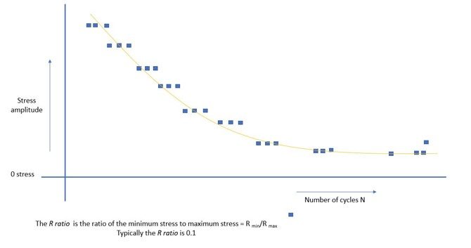
This means that to generate a run-out, or reach the endurance limit running at a frequency of 25Hz (25 cycles/second), one test will take around 4½ days. It is usual to perform at least two repeat tests. This means that, when generating a stress life fatigue curve (figure 1), this one stress level on the curve could take around 13 days to generate, assuming 24/7 operation of the test machine.
In practice, as the stress intensity rises, the cycles to failure will reduce (as figure 1 illustrates). Nevertheless, this does demonstrate how machine-intensive fatigue testing can be.
Background to stress-life fatigue testing.
Fatigue cracks normally appear after multiple application and removal of a load (or an induced stress). This load can be much lower than the actual static strength. The cracks nearly always initiate at the surface, which can be the region of highest bending. They tend to propagate at 90o to the load axis.
The premise for carrying out the fatigue test is:
- The manufacturing of the samples or coupons is to the highest standard with regards to machining, drilling and utilising location jigs/fixtures. This ensures repeatability.
- A filleting tool forms the fillets on adhesively bonded coupons for consistency. A high proportion of the joint strength is contained within the fillet.
- Consistent mixing of the adhesive. The mixing should give an even distribution of the glass beads used to control bond line thickness throughout the joint.
- Clamping or locating the sample within the load frame does not impose a stress imbalance with the joint.
While every effort should go into making consistent coupons, the alignment of the test machine, grips or load train within it, are equally important. No matter how much care you take with manufacture, a poorly aligned sample could experience a higher stress in one region. This is likely to initiate a crack prematurely, thus generating a low fatigue life and scatter in the data.
The whole point of applying discipline to every stage of producing the fatigue curve is to measure the intrinsic fatigue life of the joint. It’s not a measure of poor manufacturing practice or a poorly aligned test frame or load train. Scatter in the data means we have no confidence in the true fatigue life, and so additional testing is required.
Constant amplitude stress-life fatigue test pieces.
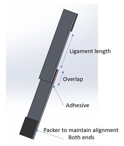
The constant amplitude stress life fatigue curve is the simplest form of fatigue testing. It represents a large part of all fatigue testing carried out today and is comparatively easy to perform and understand. The geometry typically used for adhesives within the automotive industry is a simple joint. An example is the lap shear joint, Figure 2.
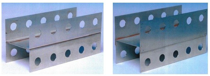
However, ISO/TR 12998:2019 references T-peel, Top hat and the H structure geometries. The H Structure is complex, requiring specialist grips and alignment couplings. Previous trials with this part highlighted problems with uneven load take-up and premature failure, even when using precision bonding fixtures. The structure does however lend itself to both T peel and lap shear joints, as Figure 3 shows.
Tests showed that the ligament length, shown on the lap shear image in Figure 2 (on the H section it is the distance between the hole centres and the adhesive line), contributes to an uneven stress state within the structure. Consequently, any misalignment transfers directly to the bond line. The larger the ligament length, the more compliant and accommodating the structure can be. For this reason, it is important when using packers (Figure 2) to position them correctly and so maintain a consistent ligament length and level of overall compliance.
Load state.
In real life, loads and stresses are not constant. For example, a car repeatedly driving over bumpy roads and potholes would impose a very different cyclic load regime to the constant amplitude test. In addition, the final geometry of an automotive structure may also impose a very different stress state to the simple lap shear joint.
The constant amplitude test therefore typically does not simulate real time loading. It does, however, allow ranking of joining techniques, adhesive types, pre-treatments and surface preparation. The test also provides an endurance limit for design engineers. Furthermore, it’s also applicable to flow drill screws, spot welds, self-pierce rivets, and even combinations of joining techniques.
Tension-tension test.
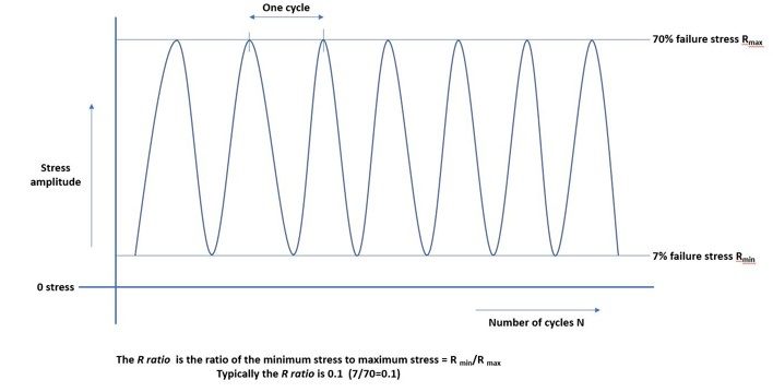
Typically, the type of fatigue evaluation employed when testing automotive adhesive joints is known as a tension-tension test. This defines the load range which will not drop below zero (or go compressive); Figure 4. The sample will always be under a tensile load, and the upper and lower loads employed will be +ve. This again simplifies the testing, because a sample that always has a tensile load will not buckle and will be easier to control.
The stress ratio that defines the test is R 0.1. This means the load/stress intensity will follow a range between:
R 0.1 = load min / load max for example, 90 and 9% of the static strength.
The static strength of the joint needs to be established prior to any fatigue testing. This is vitally important for generating the load regime and should be based on at least 5 quasi-static tests.
Additional factors to consider.
Cyclic movement of an actuator.
In a test rig this depends on many things. For example, the volume of oil required to move the actuator. Higher force actuators require larger volumes of oil (Force = Pressure x Area). Therefore, smaller actuators (smaller area/volume) are more responsive and, with a similar supply of hydraulic oil, will run at a faster frequency.
Compliance of the sample.
This is a product of your test piece design. A more compliant sample (greater movement) will require a larger movement of the actuator to impose the load regime, which will limit test frequency.
The test frequency.
Once you establish a test frequency, you should not change it. Frequency can alter crack propagation rates, so you must test all samples at the same rate. Usually, 25-40 Hz is achievable (dependent on many parameters). An additional factor that you must consider is adiabatic heating (deformation energy turns into heat). Whilst this testing is high cycle (small amplitudes), you should not assume that some displacement induced heating does not take place. Monitoring a contact thermocouple mounted adjacent to the adhesive at the chosen frequency will allow you to ensure it’s not a factor.
Oil flow.
The servo-hydraulic valve controlling the oil flow will consist of a series of ports with a spool valve that controls the oil flow to the actuator. Controlling the level of overlap covering the port means it’s possible to optimise the spool valves for a specific system. Reducing the overlap can increase the response time.
Controlling inertia.
Mounting a heavy set of grips on the end of an actuator will, in effect, add a damper to the system. This mass will generate kinetic energy, KE, dependent upon:
KE = 0.5 x m (mass) x v2 (velocity)
The actuator needs to overcome this energy each time it changes direction.
Machine control software can help to significantly reduce this effect with inertia compensation and adaptive control systems that respond to the sample compliance. With feed-back from position or load, the software can impose tight control over actuator movement. ISO 12998 defines this control as within 1% of the target stress or load level. For example, a test piece with a static strength of 10kN running at R = 0.1 at 70% would need to adhere to 7000N ± 70N at the peak load, and 700 ± 7N at the lower load.
Alignment.
Manufacturing a precision ground steel strain gauged alignment blank which replicates the test piece geometry of the lap shear specimen (or any specific design of test piece), such as shown below in Figure 5, is a useful way of checking the alignment of your sample within the load frame. This is especially true if you have custom-made grips. It does not matter that the alignment blank is machined from a material with a different modulus to the adhesively bonded sample, because the gauge is just loaded elastically to a similar load (maximum) used for generating the stress life curve.
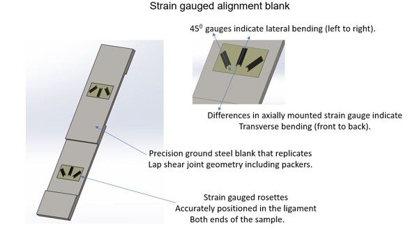
By simultaneously monitoring the gauges, you can make adjustments to bring the strains into balance within the load frame using an alignment cell (mounted under the crosshead) if fitted. You should carry out this procedure periodically, and always if you’ve changed the crosshead position.
The objective is always to eliminate as many external factors that can influence the fatigue test as possible. You want to generate confident data with the least financial waste.
How we can help you with fatigue testing.
Embarking on a programme of fatigue testing is a key step in validating material and component performance. It’s also a major resource commitment. The aluminium experts in our Materials Characterisation & Testing department can support you by organising the testing, interpreting the results and providing advice. Contact us to find out more.