
Posted on: 16th September 2016
This is the fourth post in our series of blogs about aluminium rolling process models. I’m going to use a recent case study to tell you about our coil annealing model, and how it saved one of our clients from embarking on an expensive CAPEX project.
Do we need more coil annealing furnaces?
This was the question a client of ours asked recently. He operates many different types and sizes of batch annealing furnace and capacity was becoming an issue. Consequently, he needed to know if he could improve the utilisation of his existing furnaces rather than buy new ones. To help him answer this question, he used our coil annealing model.
With guidance from the Innoval team, our client prepared an instrumented coil. This is a scrap coil fitted with an array of thermocouples in known positions throughout the coil. The instrumented coil calibrates the model via a series of trials. These trials consist of heating the coil and recording both the furnace temperatures and the coil temperature response. A separate, off‐line activity then tunes the model’s parameters so that it is able to reproduce the furnace performance.
Investigating the current practices
First of all, our client investigated one of his annealing practices which was supposed to achieve a coil temperature of 360° C with a 2‐hour soak. Two types of furnace used this practice. The newer furnaces had coilside air jets, whereas the older and smaller furnaces had air up‐flow over the coil.
Each furnace type had its own heating profile which our client believed gave him what he wanted. However, even before any productivity improvements were proposed, the calibration trials revealed that both furnace types caused the coils to overheat. Furthermore, one of them was overheating by a large amount.
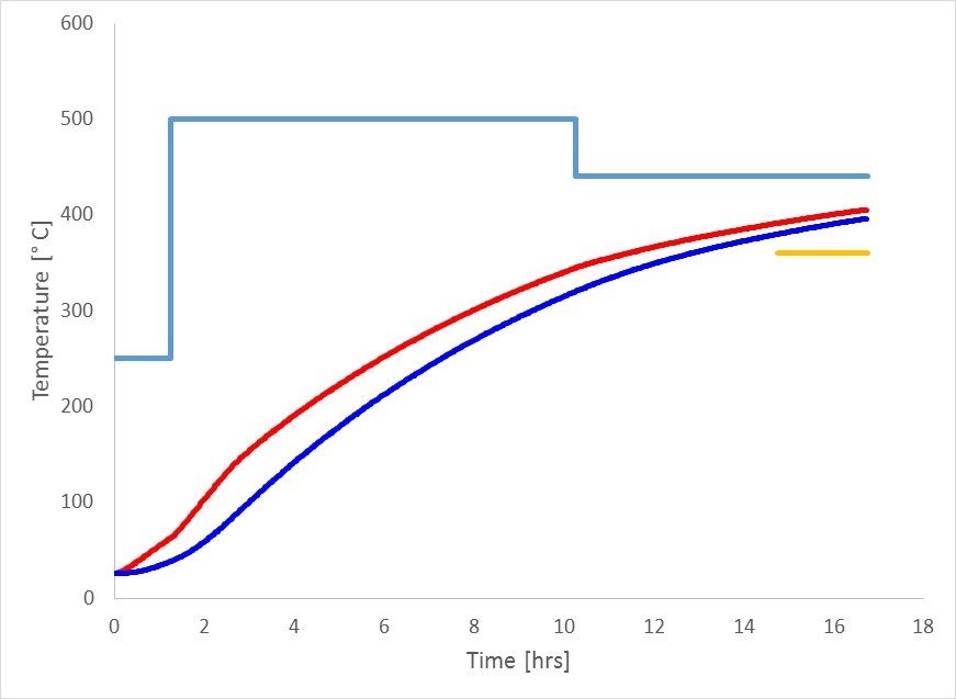
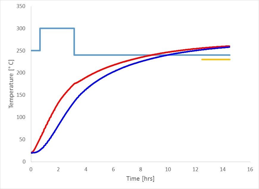
In the following illustrations, for the original heating profiles, the furnace air temperature set point is shown in pale blue. The temperature target is in yellow. The ‘leading’ coil temperature is in red, and the ‘lagging’ temperature is shown in darker blue. For the illustrations showing the improved heating profiles, the furnace temperature set point is shown in green.
The leading temperature is the maximum temperature that the model predicts anywhere in the coil at any particular moment. The lagging temperature is the corresponding minimum temperature that exists somewhere in the coil at the same time. The lead temperature is usually somewhere on the surface of the side‐face of the coil. The lag temperature is usually near the mid‐width and mid‐build‐up in the coil.
Original profiles
Figure 1 is from the furnace design which employs air jets impinging directly onto the flat side faces of the coil (approximately 8 tonne coil). We can see here that the coil exceeds the required temperature in much less than the 8‐hour cycle time.
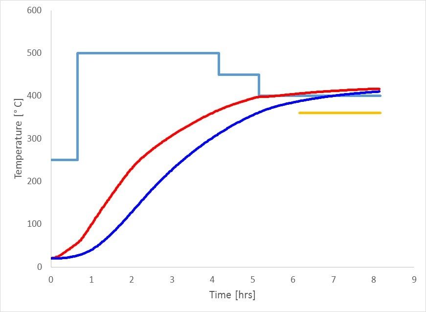
Figure 2 is from the older, but also smaller, furnace design with the heating air flowing up over the whole coil. Again, we can see that the coil exceeds the required temperature. However, in this case, in double the cycle time shown in Figure 1.
Consequently, unnecessarily long cycle times tie up the furnaces and reduce productivity. These overly long cycles are also consuming electricity and gas which add to the process costs and carbon footprint. We must also take into account the metallurgical consequences (microstructural or surface quality). However, these are more difficult to quantify immediately.
Revised profiles
Once our client had collected the temperature data and completed the model calibration exercise, he used the model to devise new heating profiles. These profiles achieved the required heating in a reduced time (Figure 3 & Figure 4).
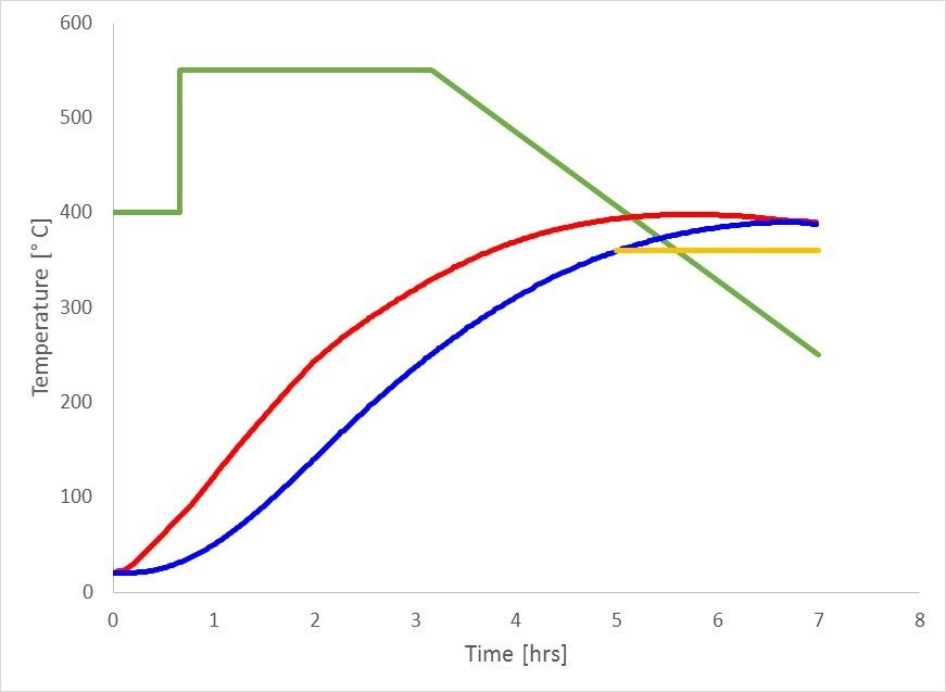
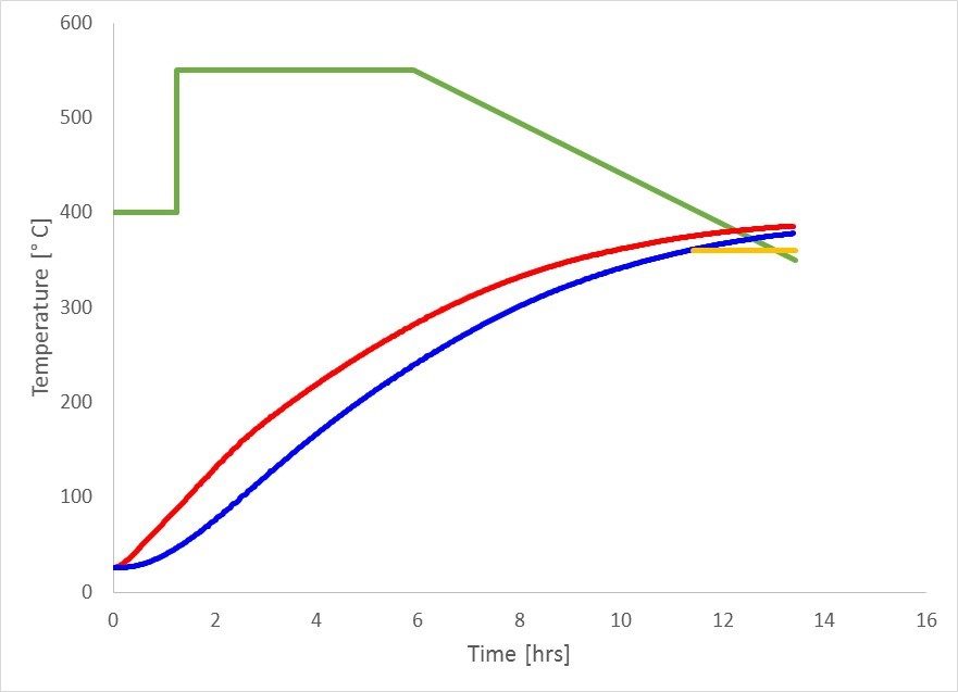
The cycle time improvements were 70 minutes and just over 3 hours respectively. Cumulatively, this represents a significant amount of additional annealing capacity (14% & 20%).
Following these successes our client investigated another annealing cycle in the side‐jet type furnace. This one was at a lower temperature of 230° C plus a 2 hour soak. He found that this heating profile was also overheating the coil. However, this time it was only by about 20° C (Figure 5).
Using the calibrated coil annealing model, our client came up with a revised heating profile. On this occasion the new cycle time saved almost 4 hours, or 26% of the original cycle time.
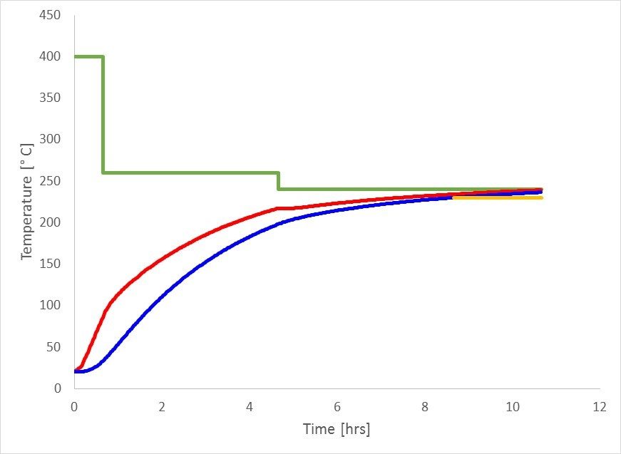
There might have been further gains too. However, due to concerns about surface staining on the coil, the middle section of the heating profile had a maximum temperature of 260° C. Without the staining concerns, the set-point could be higher, meaning the coil would reach the required temperature sooner.
Further advantages
By using a calibrated version of the Innoval coil annealing model, our client increased his productivity without buying more furnaces. He achieved this by reducing his coil annealing cycle times. However, he also gained more accurate coil temperature control and reduced operating costs. Furthermore, he now has the ability and confidence to design appropriate heating profiles for all existing practices and new coil products.
The coil annealing model I’ve described in this blog post is just one of several aluminium process models created by Innoval. We think they’re the most accurate process models available to the industry today. This is because, as well as the physics of the process, the models incorporate the comprehensive knowledge and understanding of aluminium that’s unique to us.
You can read what one of our customers says about them here, and also watch an animation of our coil annealing model.
This blog post was originally written by Andy Darby who has now left the company. Please contact Kyle Smith if you have any questions.