
Posted on: 20th July 2021
Every metallographic lab has visible light optical microscopes. In one of my previous blogs, I introduced a method of using optical microscopy to evaluate the cleanliness of an aluminium sheet surface. This method makes use of the most basic function of an optical microscope; showing the real colours of an object. It’s a simple technique, and not something you can get from an electron microscope.
In contrast to this simple way of using visible light optical microscopes, scientists from the University of Manchester have used a conventional optical microscope to perform virtual imaging at 50 nm lateral resolution (https://doi.org/10.1038/ncomms1211).
In this blog, I am going to give some examples of how we use optical microscopes at Innoval to support our commercial customers and collaboration partners.
Using optical microscopes to analyse:
1. Intermetallic particles
The type, size, shape and distribution of intermetallic particles in aluminium alloys can affect their properties. These include mechanical properties, formability, corrosion resistance, electric conductivity, etc. We can obtain a lot of information about constituent particles, and many types of dispersoids, in aluminium alloys using optical microscopes. However, most types of ageing precipitates are out of reach.
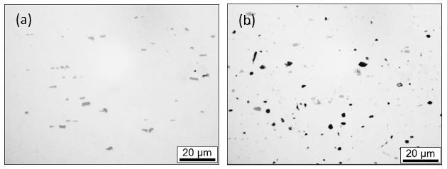
Insufficient solutionisation of some heat treatable AA6xxx aluminium alloys leaves a high population density of Mg2Si particles undissolved in the aluminium matrix. Consequently, the following ageing process is unable to strengthen the alloy to an optimal level. This is due to the lack of available solute atoms to form strengthening precipitates. Therefore, we can use optical microscopes to assess whether the solution heat treatment is optimised by characterising the number density of Mg2Si particles in the alloy. Mg2Si particles appear as dark grey spots in optical images, in contrast to light grey iron-containing particles.
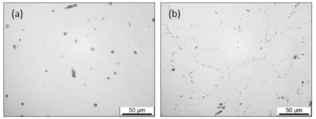
Quench rate is also a critical parameter that needs to be well controlled with AA6xxx alloys. If we do not quench the alloy fast enough, we lose alloying elements in the super saturated solid solution. These elements tend to precipitate out preferentially at grain boundaries. Unfortunately, this may lead to reduced mechanical properties, poor fracture toughness and low corrosion resistance of the alloy. However, we can use optical microscopy to assess whether the quench rate is sufficiently high by characterising the number density of grain boundary precipitates in the alloy.
2. Grain structure
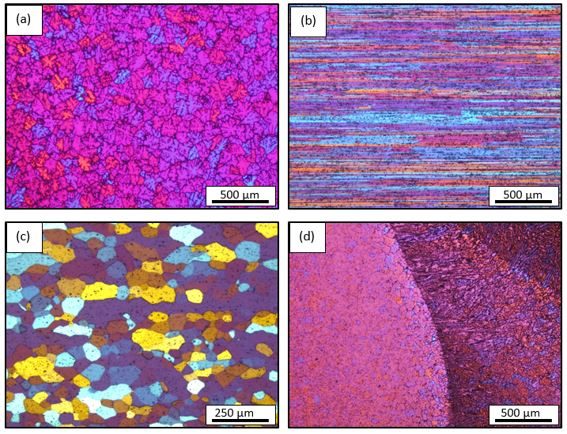
Grain size has a measurable effect on most mechanical properties of aluminium alloys. Therefore, we need to measure the grain size so as to control it and the mechanical properties. The grain structure is a result of the casting/thermo-mechanical processing/heat treatment/welding processes that an alloy goes through. Consequently, examination of grain structure can guide us in process improvement activities. Furthermore, it can help us to understand microstructural defects, such as porosity and micro-cracking.
Very often we use Barker’s anodising to prepare samples and observe the grain structure under polarised light on an optical microscope. You can read more on this subject in another of our blogs; ‘Optical microscopy to analyse aluminium alloy grains‘.
3. Surface features and defects
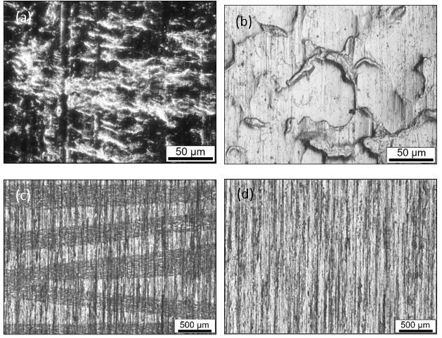
If dark field mode is available on your optical microscope, you can use it for characterising defects like cracks and porosity in your products. Dark field mode makes these features readily visible compared to the normal bright field mode. Sometimes a C-DIC insert will be very useful for characterising surface defects with very shallow profiles. Examples of such defects include Luder’s lines in 5xxx aluminium alloys.
For some high-profile surface features, optical microscopes may not have enough depth of view. However, this is not a problem for an optical microscope which has an automatic focus stacking function. On the other hand, if such a function is not available on your optical microscope, you can still easily perform focus stacking. You simply take a series of micrographs and use an app like Photoshop or ImageJ to do the job. In fact, many photographers perform focus stacking to create amazing pictures.
Above are a few examples of how we use optical microscopes in the Innoval labs. Of course, there are many other applications for optical microscopes, but I’ve not included them in this blog.
Characterising your aluminium products
The Materials Group at Innoval has a huge amount of expertise in the techniques I’ve described here, alongside many more. Furthermore, we supplement our in-house equipment with state-of-the-art equipment at leading partner universities. This means we always use the most appropriate technique to solve our clients’ problems. In fact, with our extensive in-house characterisation and analysis capabilities, we can usually get to the bottom of most metallurgical and surface problems.
Finally, Materials characterisation and testing are just some of the topics we cover in our Introduction to Aluminium Metallurgy Training Course. This live online course takes place over 3 half-day sessions (10.5 hours), and we run it several times a year. Please keep an eye on the page in the link above for the dates of the next course.