
Posted on: 1st June 2018
This is the first part of a two-part series on process modelling. In this blog I will describe what’s important for plant capacity modelling. In part two I will talk about energy utilisation modelling.
One of the cornerstones of process modelling is mass continuity and energy balances. In other words “what goes in comes out, unless it stays there”.
Inherent in the basic premises and calculations is a notional time-base. This might be ‘per hour’ or ‘per year’ for example. Using these time-bases then allows us to consider the basic quantities of mass and energy in terms of flows, e.g., ‘tonnes per annum’ or ‘kWh’ etc. Immediately the ability to investigate process (and plant) throughputs and capacities then becomes apparent.
I will discuss in this blog how we utilise these metrics in plant capacity modelling. They are integral components of Innoval’s process cost modelling approach which we apply to many process and plant scenarios (new and existing). I will not describe any particular process, but instead I’ll illustrate the principles we generally apply to plant capacity modelling.
A hypothetical plant
Consider a plant that comprises a set of separate processes. Each of these could form part of a process sequence for the manufacture of the required products. Some products may need to use all the available process steps; others may bypass some processes. The number of products, each defined by characteristics such as size, shape, properties etc. is, in principle, limitless. An illustrative plant consisting of 7 processes (‘A’ to ‘G’) is shown in Figure 1:
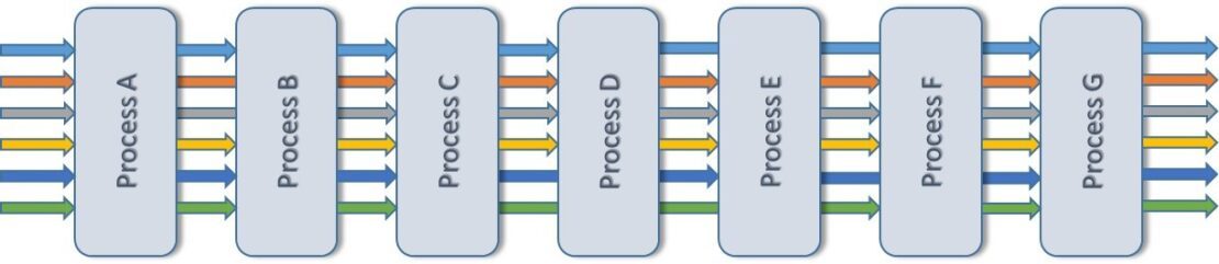
This particular plant is currently producing 6 different products. You can see the process flow of each represented by a different coloured arrow.
For purposes of simplification and illustration, I’ve ignored added complexities such as process losses, waste disposal and internal scrap recycling flows.
With a hypothetical plant now established, we can start to think about plant capacity modelling.
The components of plant capacity modelling
Calculating the plant capacity is often not as simple as reading the rated capacity (the ‘boilerplate’) on the side of the equipment. To use an automotive analogy, just because the speedometer on the vehicle indicates a maximum of 150 mph, it doesn’t mean that the vehicle can achieve that speed – or would it be wise to even try! Furthermore, the plant capacity isn’t the sum of the all the constituent process capacities, except in very specific cases. Indeed, as with a chain, the plant capacity will be governed (most likely) by the weakest link. This is the ‘bottleneck’ process, i.e., the process with the most limitations and lowest production capability.
Essentially there are three factors that determine the production capacity of each process, and hence that of the plant overall. These are (1) the process uptime, (2) the mix of products, and (3) the process (productivity) efficiency for each of the products making up that mix. You must evaluate each and then combine them to produce the process capacity. Each of these three categories will be considered below:
Uptime
In principle each process would be available for work at all times that the plant is open for business. In reality, there are several reasons why this doesn’t happen. Three such reasons are given below:
Planned downtime

There are portions of time when equipment needs to be taken out of operation for essential maintenance and repairs. We often refer to this as ‘planned’ downtime. It is important because equipment and components will wear out.
Well-targeted maintenance and replacement programmes can usually help avoid catastrophic (and more expensive or dangerous) events.
Unplanned downtime
Sometimes there are the unforeseeable occurrences. These are the breakdowns (equipment or component failures) and other factors that bring operations to an immediate halt. We often refer to these as ‘unplanned’ downtime. Extensive and carefully executed preventative maintenance programmes aim to reduce this type of downtime.
Changeover downtime
Where a plant makes multiple products, from time to time each process will need to alter its feed materials and, probably, its operating conditions. These alterations are rarely instantaneous. Particularly in batch or semi-batch processing industries, such as aluminium rolling and finishing, these changeovers may take minutes, but could also last for many hours. This is especially true if the ‘changeover’ includes the time it takes to reach a new operating steady-state process condition.
In process modelling or production planning, you can budget for each of the types of downtime. Plants can do this by setting fixed maintenance schedules. They can also analyse process history data for unplanned lost time and changeover efficiency.
You can express downtime in absolute terms (hours) or as a percentage of the total operating time available.
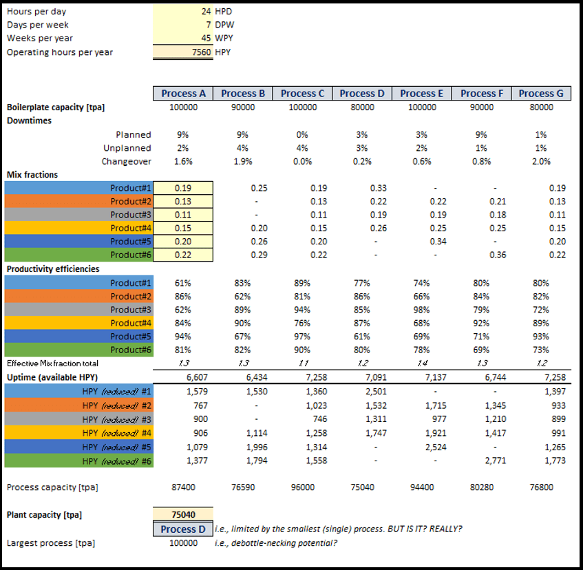
‘Uptime’ (available hours per year) is what remains after we’ve taken all these deductions away from the total available operating hours. For the plant example we’re looking at here, I’ve evaluated the process uptime (actually expressed in terms of downtimes in this illustration) in Figure 4 below.
Product mix
In all but the simplest process plants, production is about realising multiple products, either in parallel or sequentially. In the illustrative example created here, the plant comprises a sequence of processes. Furthermore, I’ve arbitrarily defined the product mix at the input to the first process step ‘Process A’. As an alternative, it is often preferable to define the final (output) product mix instead.
The product mix is the mass fraction of each product as part of the total input (or output). The sum is unity. By the nature of the sequential process arrangement, we can then also determine the input mass fractions to each subsequent process step. This is quite simple if there are no losses, but more complex if there are variable material losses in the preceding process. For the purposes of this example, I’ve assumed zero material losses. An example is shown of ‘Mix fractions’ progressing through the plant in Figure 4:
Productivity
Although the individual processes may be easily identifiable pieces of equipment, such as a rolling mill or a furnace, it’s likely that each process will have multiple operating ‘modes’. This means there will be different operating conditions for each product. These modes might manifest as different speeds, temperatures or configurations. These process settings reflect the required properties of the product. They could be the dimensions (length, width, thickness), material properties (strength, composition), or some product quality requirement (surface finish, temperature history, dimensional uniformity).
Taken together, all these competing requirements have the same effect. They combine to give rise to a process ‘efficiency’ factor. In other words, usually a reduction in how much that process can actually produce compared to its theoretical or design (‘boilerplate’) capacity. It seems to be extremely rare to encounter a combination that increases the rated process capacity. However, this is possible of course.
Productivity efficiency factor
In the simplest terms, the productivity efficiency factor describes the way in which any particular product is less (or more) easy to make than an ideal case. Consequently, there’s increased (or decreased) time required to process a given input mass. I’ve included a set of hypothetical productivity efficiency values in Figure 4 above. I’ve also shown values for products not being processed through particular process steps. This is to illustrate that where the particular process is optional, we may already know the efficiency factor and that it is part of the process knowledge mapping database.
A summation of all the input product mix fractions and productivity efficiency ratios gives rise to an effective product mix ratio. If every product could be made at the same rate and process conditions, for example speed etc., then this ratio would also be unity. Values greater than one indicate that it will take longer to make the product mix.
Machine time by product
For many reasons, but primarily for aiding calculation of energy and utility consumptions, the number of machine hours required to realise each product at each process stage is necessary. I’ve shown a formula for calculating these machine times in Figure 5:
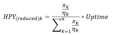
where Xk is the mass fraction of product k, nk is the production efficiency of product k, n is the number of products being realised by that particular process, and Uptime is the available operating hours for that same process.
You can see illustrative results in Figure 4 labelled as rows ‘HPY (reduced) #1’ through to ‘HPY (reduced) #6’.
Calculation of Plant capacity
In contrast to the relative complexity of determining the machine hours by product, you might expect the plant capacity calculation to be easy. The boilerplate capacity of each process is scaled by multiplying by the ratio of ‘Uptime’ and ‘Operating hours per year’. This gives the capacity of each process (tonnes per annum for example). The plant capacity would then be the minimum of these individual process values. For example, according to the example shown in Figure 4 above, this is 75040 tonnes per annum and with ‘Process D’ being the limiting process. However, in the type of interconnected process configuration described here, that would be wrong.
The weakest link in plant capacity modelling
The correct approach for plant capacity modelling requires that we assess the weakest link in the process chain for each product. However, you must note that not all products utilise each process step. In a close-coupled process chain such as that illustrated here, a further detail is that no process can create material. The mass throughput can only be up to and equal to the flows in the preceding processes. This must account for the effect of enforced material losses of course which are assumed to be zero in this simplified example.
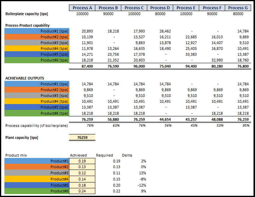
The net result is that some processes may be unable to achieve anything close to their boilerplate capacity. For example, ‘Process C’ in Figure 6, even though all products go through it, is at 76% of its maximum rated capacity. Other processes, such as ‘Process E’ in Figure 6, may appear even further under-utilised. However, it is essential to realise that we’re processing only 4 of the 6 products here.
Now we can correctly determine the plant capacity by summing the output of each product from the last (final) process each encounters. In this example, that is ‘Process G’.
In this example, the achievable plant capacity is actually greater than the obvious choice described above. However, it might not always be so.
One of the unavoidable problems with these process-based constraints is that the initial product mix might alter. The process and plant configuration will determine how much this affects the calculations.
De-bottlenecking
A simple tabulated view of the plant in a process-by-process way allows us to clearly identify the rate-determining step (as shown in Figure 6 above).
By reference to Figure 4 (part of the same worksheet as Figure 6), it also allows more immediate targeting of the best means of improving production capacity. For example, are there large amounts of unexpected downtime that need reducing? Or is it primarily a capacity constraint imposed by having, for example, only one piece of equipment at a particular process step? Installing an additional piece of equipment multiplies the ‘boilerplate’ capacity of course.
If you have any questions about plant capacity modelling or any of the topics described in this blog, please drop us a line. Perhaps you’re considering doing your own plant capacity modelling? In which case we can help you.
This blog post was originally written by Andy Darby who has now left the company. Please contact Kyle Smith if you have any questions.