
Posted on: 16th August 2023 by Dr. Ceri Williams
Aluminium alloy development is a dynamic field, with active research across many sectors all over the world. Regardless of whether the end use is in packaging, structural or battery conductor foil, our clients often enlist our help to design new alloys with specific property requirements. They rely on our ability to link together our understanding of composition, processing and microstructure, to produce a material with the right balance of features.
Historically, new alloys were developed based on trial and error, often casting large volumes of metal in order to ‘strike lucky’. At Innoval, we believe in a more targeted approach. We have recently invested in thermodynamic software which, together with our experience, allows us to accelerate the alloy design process. Furthermore, access to off-line processing through our partner network, and extensive in-house characterisation facilities, mean we can offer the complete alloy development package.
Software to support alloy development.
Numerous software packages utilise the CALculation of PHase Diagrams (CALPHAD) approach to thermodynamic modelling. Examples of commercially available software that contain thermodynamic models to generate equilibrium phase data include Pandat (by Computherm LLC), Factsage (by Thermfact Ltd. and GTT-Technologies) and Thermo-Calc Software.
The software allows for the calculation of:
- Solidification properties
- Phase equilibria
- Phase transformations
- Thermo-physical and physical properties
- Mechanical properties
Predictions made using these software packages will assume that the phases present in the alloy will be the most thermodynamically stable equilibrium phases.
Applying the models to aluminium.
During most standard aluminium production routes, the main phases that strengthen an aluminium alloy will be metastable non-equilibrium phases. This is because the alloying elements (Mg, Si, Cu etc.) need time to diffuse through the aluminium matrix to form these equilibrium phases i.e., reaction kinetics. JMatPro® by Sente Software uses a combination of thermodynamic and kinetic databases to improve the phase predictions. Therefore, it can account for both the stable and metastable phases. For this reason, Innoval uses JMatPro®. The software is versatile in that predicts solidification properties which occur in non-equilibrium conditions. However, it also predicts the boundaries of different phase fields for equilibrium conditions.
An example using AA6061 – optimising composition.
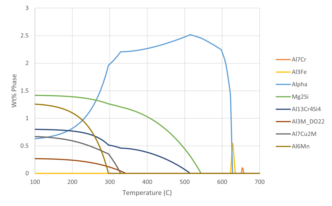
Figure 1 shows an example of the thermodynamically predicted equilibrium phases generated by JMatPro® for a AA6061 alloy. We can see the variation in the equilibrium phases at a given temperature as a function of %Mg across the allowable range of %Mg for the alloy specification. Knowing what phases should be present allows us to predict the type of microstructure and, therefore what type of properties, the alloy might have. For a given %Mg, we can more easily read the exact proportion of each phase across a range of temperatures from Figure 2. Furthermore, this can be verified experimentally, and we’ll cover this later.
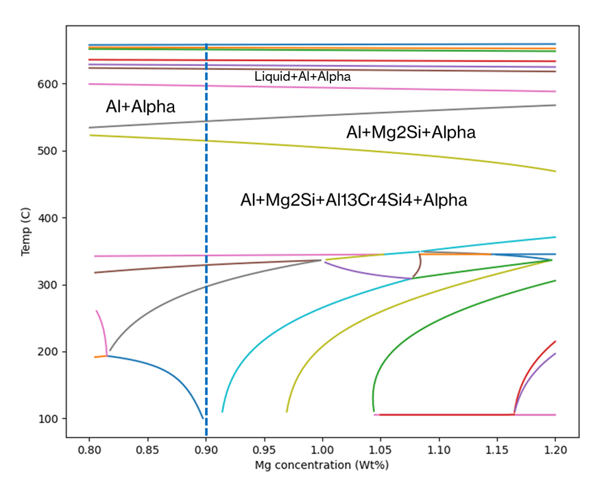
It is possible to use the type of information in Figure 1 and Figure 2 to pre-screen vast numbers of potential candidate compositions in an alloy development project. In addition, it would be possible to predict the phase stability as a function of chemistry and temperature for each one. This allows us to discover chemistries that are more likely to meet the target property requirements of the alloy. Finally, we can explore trade-offs between the target properties and the alloy composition, thereby allowing for cost and/or process optimisation.
An example using AA6061 – optimising processing parameters.
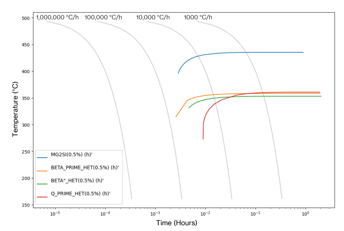
Once we’ve decided upon a base alloy composition, cooling curve transformation calculations can help to identify critical cooling rates. This is to avoid equilibrium or metastable precipitation during quenching from solution heat treatment. These calculations also ensure we get the best properties.
We can generate time-temperature transformation curves that identify temperature/time combinations that provide optimum strengthening. In the AA6061 CCT curves generated at Innoval using JMatPro® (Figure 3), we can see that we need a quench rate of just under 28°C/sec to avoid the formation of secondary phases during quenching.
However, the outputs of the software cannot be interpreted in isolation. It is important to understand the limitations of the phase predictions and make recommendations accordingly. The software will make some assumptions about the kinetics of the alloy system in question. Therefore, it is essential that the model is validated to ensure that those assumptions are applicable to the alloy under investigation.
Validating the model predictions.
Aluminium alloy processing is a complex multi-step process. Unfortunately, it is impossible to deduce from a review of the material properties measured at the end of production whether the alloy truly reflects the predictions of the thermodynamic model.
Experimental verification of the process on a step-by-step basis helps to validate the model’s predictions. This should give us confidence that we’ve found the optimum alloy composition. There are many quick and accurate thermal analysis experiments that we can do at Innoval’s in-house laboratories. These experiments cover many aspects of the alloy development process:
- Solidification and melting studies
- Homogenisation and solution treatment studies
- Precipitation and second-phase particle studies
Differential scanning calorimetry.
Differential scanning calorimetry (DSC) is a powerful technique to support alloy development. Figure 4 shows a schematic representation of the heat-flux differential scanning calorimeter (DSC).
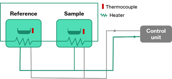
Essentially, the equipment works by measuring the energy required to keep a small (~10mg) sample and an empty reference pan at the same temperature. The sample is heated at a constant rate. When a reaction occurs in the metal (e.g., melting or a phase transformation or the formation/growth of secondary phases) the calorimeter must supply more energy to one furnace than the other to balance out the reaction and keep the temperature constant.
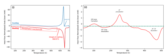
Figure 5 shows an example of the heat-flow trace that is produced from a DSC experiment. Figure 5(i) shows the full trace. Here, the sample has been heated from room temperature to 700°C at 20°C/min, then cooled back down at the same rate. The major observable peak relates to the melting/solidification of the core alloy. The signal is affected by the underlying differences between the sample and reference pans, and this creates a ‘baseline profile’. By subtracting the baseline profile, which you can see in Figure 5(ii), we can identify the peaks that correspond to the formation of metastable hardening phases. The troughs relate to the dissolution/melting of the second phase particles. It is these signals that give us insight into the various aspects of the microstructure, as described below.
Melting point studies.
The onset of melting of the core alloy (indicated in Figure 5) can be compared to the solidus temperature ranges predicted by the thermodynamic software. Kolb et al. [1] compared the solidus predictions from three commercially available CALPHAD databases/software packages to the DSC measured onset of melting for an AA7075 alloy variant. We’ve combined this data with predictions from JMatPro® (conducted at Innoval) and compared them in Figure 6. For a given alloy, there can be significant variation between the predicted and measured solidus temperature. Therefore, the validation experiment is essential.
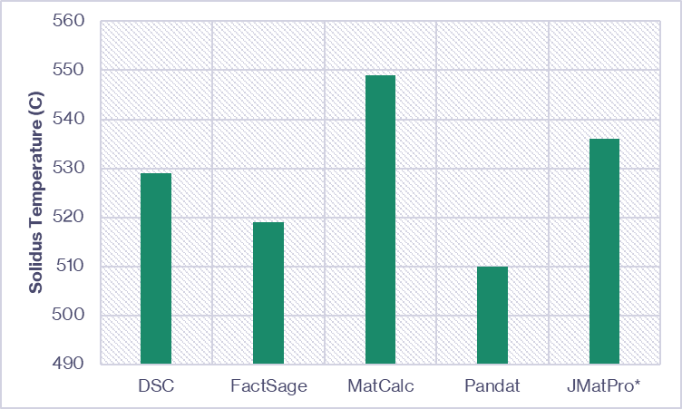
with *data generated at Innoval using JMatPro® V13.2.
Homogenisation.
The purpose of homogenisation in aluminium processing is to redistribute the alloying elements from the as-cast structure. As a result, the homogenised material is more amenable to subsequent processing. In the case of 7XXX alloys, a critical function of the heat treatment is to allow for the dissolution of the low-melting point phases (commonly η and S). This is because they can lead to incipient melting if they remain in the microstructure.
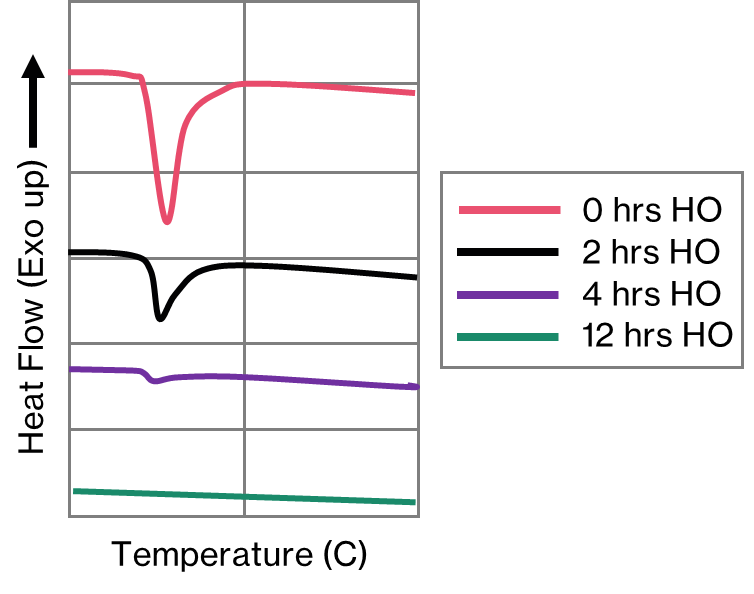
The thermodynamic predictive software will suggest an appropriate temperature for homogenisation by calculating the solidus for the phases of interest. The DSC validates that temperature by allowing us to measure the onset of melting of the phase from the appropriate endothermic peak that appears on the DSC trace. Furthermore, we can establish the time taken for the complete dissolution of these phases experimentally. Wozniki et al. [2] demonstrate this by conducting a DSC experiment after incrementally increasing homogenisation times. In Figure 7, the peak corresponding to the low melting point phase gets progressively smaller as the homogenisation time increases, until the process is complete. Consequently, it’s possible to make significant cost and productivity savings by ensuring that homogenisation does not go on longer than is absolutely necessary.
It’s important to note that DSC requires a certain threshold volume of a phase for a signal to be recorded. Therefore, it is advisable to conduct a microscopic examination of the material to confirm that all phases have gone into solution.
Secondary phases.
DSC can detect the formation of second phase particles/precipitates, as seen in Figure 5(ii). However, you must have some prior knowledge of the expected phases to be able to correctly identify the peaks corresponding to precipitation. Therefore, this technique in isolation is not appropriate to verify whether the predicted phases were formed during alloy production.
Scanning electron microscopy (SEM) combined with semi-quantitative energy-dispersive x-ray (EDX) analysis allows us to identify the composition of particles down to <1µm. Automated scanning and analysis of large areas of the microstructure can give a representative view of the phases present in the alloy. This provides a basis for a statistical review of the particles present. We can then compare the proportions of phases to predictions similar to the example in Figure 2. Consequently, we can have confidence in the model predictions.
In conclusion, the powerful combination of thermodynamic modelling/phase prediction and materials characterisation makes alloy development cost and time efficient. At Innoval we can help to meet or even exceed the target properties of your alloys. If this sounds interesting and you’d like to know more, please contact us.
References.
| [1] | G.-H. Kolb, S. Scheiber, H. Antrekowitsch, P. Uggowitzer, D. Pöschmann and S. Pogatscher, “Differential Scanning Calorimetry and Thermodynamic Predictions—A Comparative Study of Al-Zn-Mg-Cu Alloys,” Metals, pp. 6, 180., 2016. |
| [2] | A. Woźnicki, B. Leszczyńska-Madej, G. Włoch, J. Grzyb, J. Madura and D. Leśniak, “Homogenization of 7075 and 7049 Aluminium Alloys Intended for Extrusion Welding,” Metals, pp. 11, 338., 2021. |