
Posted on: 29th June 2018
This blog follows on from my previous one about plant capacity modelling. This time I’m going to talk about energy utilisation modelling.
Process cost modelling is just one of the modelling services we’ve developed for our clients. Our models incorporate Innoval’s knowledge and experience of the global aluminium industry. Therefore, even if you’re new to aluminium, you can trust our models to give you unbiased and reliable information.
A hypothetical plant
Last time I introduced a hypothetical plant consisting of 7 processes producing 6 different products. Without doubt, this process sequence will also require energy to operate. Some, or all, of the plant will require the provision of various external services too. You can see the complete plant (in simplified form) in Figure 1:
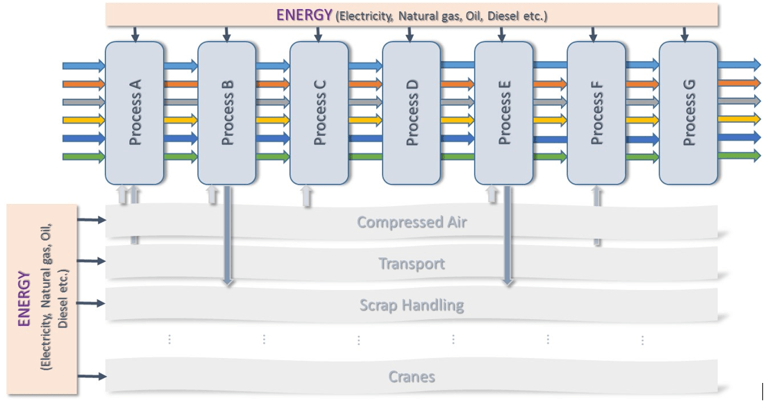
For purposes of simplification and illustration, I’ve ignored added complexities such as process losses, waste disposal and internal scrap recycling flows.
With a hypothetical plant now established, we can start to think about energy utilisation modelling.
Inputs for energy utilisation modelling
An understanding of what each process is making, when and how it is making it, is key to evaluating the consumption of all the materials the plant needs to achieve its purpose. In the aluminium industry, many of the processes involve heating and cooling large masses of metal. It’s not surprising then, that these processes consume large amounts of energy (usually predominantly electricity and natural gas).
Below you’ll see two examples of energy utilisation; one for electricity and one for natural gas. However, the calculation process is the same for each and would be very similar for the consumptions or utilisations of all other plant feedstocks.
Energy inputs
It’s easy to assume that, because a piece of process equipment has a very large motor or heating device, it operates at the full (rated) capacity all the time. Undoubtedly there are plenty of examples where this is the case. However, in the vast majority of processes encountered in batch and semi-continuous plants, the nature of operations and process control systems dictate that consumptions are discontinuous and rarely at steady-state.
The plant energy utilisation profile is a time-based aggregation of all the energy consumptions within the plant. From such an analysis, we can identify periodic usage. We can also work out mean usage and peak loading requirements. These are essential for sizing the external supply provision. This often leads to a voltage and/or cable size specification, or pipe diameter and/or supply pressure requirement.
Additional services
Once again, we will use a process-based approach. Our list of processes can now include those additional ‘site-wide’ services that are necessary even though not directly involved with making products. These include transport, scrap management, compressed air generation etc.
Establishing a time base
For each process we must establish a time base. This can be hourly, weekly etc. However, it must be something that suits the time frame of the production process and allows sufficient granularity i.e., ability to capture changes in usage rates. In this illustrative plant, I’ve chosen a period of 24 hours, in 1 hour segments.
Normally, we’d use the in-process production sequence for the desired product mix as the means of determining the hourly consumption rates. This is one of the manifestations of the productivity efficiency factors I spoke about in my previous blog. Each product might have its own operating mode on a particular process, giving rise to varying consumption rates of energy. For example, speeds or temperatures may change depending on what is being made.
In this illustrative example, I’ve assumed that all the products consume energy in the same manner in the same process step. However, I have included variation between processes.
Electricity utilisation
I’ve constructed a series of hypothetical consumption profiles for electricity consumption. You can see them in Figures 2 and 3 below:
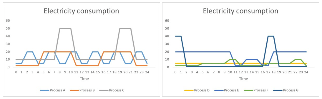
These show the cyclic consumptions typical of electric motors being switched on and off, or put under load periodically. The magnitude of the ‘peaks’ is proportionate to the size of the electrical device, e.g., motor rating [kW] or electrical heater size.
The myriad of electricity consuming devices around the plant all have their own profiles and some may be interlinked. For example, if ‘a’ happens, then ‘b’ & ‘c’ occur as a consequence. Such apparently random events in production cause changes in the wider plant consumption profile.
When superimposed, by synchronising the time steps, we can aggregate the consumption rates to give the total consumption rate profile. This is the solid red curve in Figure 4 below:
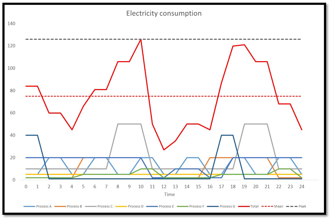
Depending on purpose, the average consumption rate might be of interest (dotted red line). Alternatively, the peak loading (dotted grey line) may be just what is required to commence discussions with the local utility company.
Although beyond the scope of this blog, the magnitude of the consumption profile (peak to trough) may also be of interest to the utility provider. It could influence the provision of suitable step-down transformer sub-stations and switchgear designs. In theory, this could mean that available utility supplies dictate production schedules to avoid outages in the surrounding neighbourhoods.
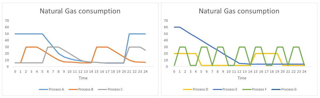
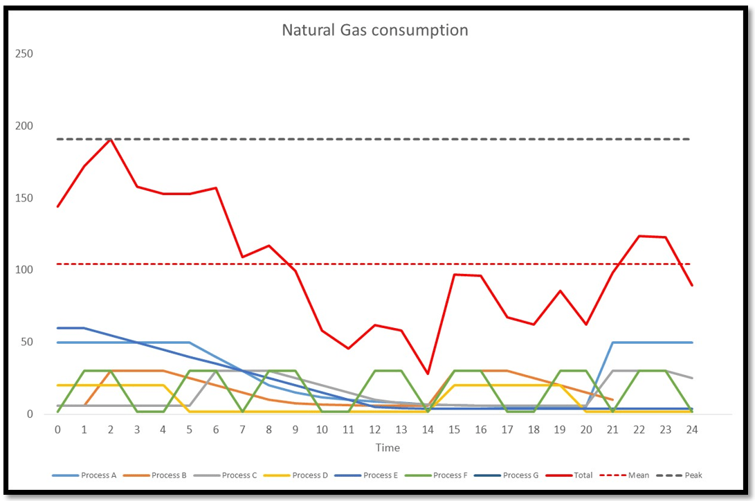
Natural gas utilisation
As for electricity consumption profiles, layers of process gas consumptions can be collated. Often the shapes of the consumption curves are different, especially where there are gas-fired furnaces. They often tend to exhibit time-decaying usage profiles reflecting the furnaces approaching target temperatures. You can see examples of this in Figures 5 and 6.
Unlike electrically heated devices (commonly ‘on-off’ type control schemes), gas-fired furnaces have PID-control applied to the gas flow control valves (even if only P or PI control strategies are actually used). Consequently, they produce different shaped response curves.
Nevertheless, the periodicity and process event sequencing causes a particular utilisation curve (solid red curve in Figure 7) to evolve. Exactly the same considerations arise for natural gas as were highlighted for electricity. The peak loading and the peak-trough magnitude may have further ramifications for supply and perhaps for plant operations.
Powerful analytical tool
Clearly the superimposition of the consumptions of multiple processes, each with varying time-bases, is not a trivial exercise. However, it’s one we can readily address with energy utilisation modelling.
The combination of material flow profiles (for plant capacity purposes) and input material flow (energy and all other materials consumed) profiles makes for a very powerful plant and process analytical tool. In fact, I’d say it’s critical for identifying cost improvement opportunities, de-bottlenecking opportunities, opportunity cost evaluations etc.
Energy utilisation modelling is an integral component of Innoval’s process cost modelling approach which we apply to many process and plant scenarios. If you have any questions about energy utilisation modelling or you’d like help doing your own, please drop us a line.
This blog post was originally written by Andy Darby who has now left the company. Please contact Kyle Smith if you have any questions.